在继续学习DRO之前,继续拓展对于Linear Programming 的知识。传统上“Linear Programming”是线性的,那么我们想让一个问题“less linear”, how should we make it ?
这一章节与“robust” 无关
Recall standard form of LP:
min c T x s.t. A x = b x ≥ 0 \begin{aligned}
& \min & & c^T x \\
& \text{s.t.} & & Ax = b \\
& & & x \geq 0
\end{aligned}
min s.t. c T x A x = b x ≥ 0
如何在这个模型中引入”非线性“?
conic linear programming,选择在相对简单易处理的 ”x ≥ 0 x\geq0 x ≥ 0
Q: Is this the only definition we can use to compare 2 vectors? Let us investigate the propoerties of the realation "≥ \geq ≥
"≥ \geq ≥
Reflexivity: u ≥ u u\geq u u ≥ u ∀ u \forall u ∀ u
Anti-symmetry:
u ⩾ v v ⩾ u } ⇒ u = v \left.\begin{array}{l}
u \geqslant v \\
v \geqslant u
\end{array}\right\} \Rightarrow u=v u ⩾ v v ⩾ u } ⇒ u = v
Transitivity:
u ⩾ v v ⩾ w } ⇒ u ⩾ w \left.\begin{array}{l}
u \geqslant v \\
v \geqslant w
\end{array}\right\} \Rightarrow u \geqslant w u ⩾ v v ⩾ w } ⇒ u ⩾ w
Homogeneity:
u ⩾ v α ⩾ 0 } ⇒ α u ⩾ α v \begin{aligned}
& \left.\begin{array}{l}
u \geqslant v \\
\alpha \geqslant 0
\end{array}\right\} \Rightarrow \alpha u \geqslant \alpha v \\
&
\end{aligned} u ⩾ v α ⩾ 0 } ⇒ α u ⩾ α v
Additivity:
u ⩾ v w ⩾ z } ⇒ α u + w ⩾ α v + z \begin{aligned} & \left.\begin{array}{l}u \geqslant v \\ w \geqslant z\end{array}\right\} \Rightarrow \alpha u+w \geqslant \alpha v+z & \end{aligned} u ⩾ v w ⩾ z } ⇒ α u + w ⩾ α v + z
These 5 properties can help us prove Farkas Lemma and then prove "Strong Duality"
Consider
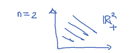
K = { x ∈ R n : x i ⩾ 0 ∀ i } = R + n \begin{aligned}
K & =\left\{x \in \mathbb{R}^n: x_i \geqslant 0 \forall i\right\} \\
& =\mathbb{R}_{+}^n
\end{aligned}
K = { x ∈ R n : x i ⩾ 0 ∀ i } = R + n
x ⩾ 0 ⇔ x ∈ R + n x \geqslant 0 \Leftrightarrow x \in \mathbb{R}_{+}^n x ⩾ 0 ⇔ x ∈ R + n L P LP L P
This is a closed set. Moreover, this is also a "pointed cone".
Ponited Cone:
Closed under addition: K ≠ ϕ K \neq \phi K = ϕ u , v ∈ K ⇒ u + v ∈ K u, v \in K \Rightarrow u+v \in K u , v ∈ K ⇒ u + v ∈ K
Conic: u ∈ K , α > 0 ⇒ α u ∈ K u \in K, \alpha>0 \Rightarrow \alpha u \in K u ∈ K , α > 0 ⇒ α u ∈ K
Pointedness: u , − u ∈ k ⇒ u = 0 u,-u \in k \Rightarrow u=0 u , − u ∈ k ⇒ u = 0
很显然R + n \mathbb{R}_{+}^n R + n
We have 2 questions:
Is "≥ \geq ≥
Is R + n \mathbb{R}_{+}^n R + n
The answer is NO !
Examples:
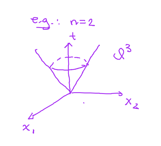
Lorentz Cone / Second-order cone:
Q n + 1 = { ( t , x ) ∈ R × R n : t ⩾ ∥ x ∥ 2 } Q^{n+1}=\left\{(t, x) \in \mathbb{R} \times \mathbb{R}^n: t \geqslant\|x\|_2\right\} Q n + 1 = { ( t , x ) ∈ R × R n : t ⩾ ∥ x ∥ 2 }
Claim: Q n + 1 Q^{n+1} Q n + 1 i n t ( Q n + 1 ) ≠ ∅ int(Q^{n+1})\neq \emptyset i n t ( Q n + 1 ) = ∅
Define: Consider the order ⪰ Q n + 1 \succeq_{Q^{n+1}} ⪰ Q n + 1
( t , x ) ⪰ Q n + 1 ( s , y ) ⇔ ( t − s , x − y ) ∈ Q n + 1 (t, x) \succeq_{Q^{n+1}}(s, y) \Leftrightarrow (t-s, x-y) \in Q^{n+1}
( t , x ) ⪰ Q n + 1 ( s , y ) ⇔ ( t − s , x − y ) ∈ Q n + 1
Exercise: E $\succeq_{Q^{n+1}} $ is a good order.
Semidefinite Cone: K = S + n = { Y ∈ S n : u ⊤ Y ˉ u ⩾ 0 ∀ u ∈ R n } K=S_{+}^n=\left\{Y \in S^n: u^{\top} \bar{Y} u \geqslant 0 \forall u \in R^n \right\} K = S + n = { Y ∈ S n : u ⊤ Y ˉ u ⩾ 0 ∀ u ∈ R n }
S + n S_{+}^n S + n 0 ∈ S + n 0 \in S_{+}^n 0 ∈ S + n int ( S + n ) ≠ ϕ \operatorname{int}\left(S_{+}^n\right) \neq \phi i n t ( S + n ) = ϕ Consider the order " ⪰ S + n \succeq_{S_{+}^n} ⪰ S + n
x ⪰ S + n y ⇔ x − y ∈ S + n x\succeq_{S_{+}^n} y \Leftrightarrow x-y \in S_{+}^n
x ⪰ S + n y ⇔ x − y ∈ S + n
With a closed pointed cone K K K O O O
\begin{align}
& \inf_{x}
& & \langle c, x \rangle \tag{P} \\
& \text{s.t.}
& & \langle a_i, x \rangle = b_i, \\
& & & x \in K
\end{align}
Here, ⟨ ⋅ , ⋅ ⟩ \langle \cdot , \cdot \rangle ⟨ ⋅ , ⋅ ⟩
Similar to the traditional LP , the conic linear programming has a dual problem:
\begin{align}
\tag{D}
& \text{Sup} & \sum_{i=1}^{m} b_i y_i & \text{ where } b, y \in \mathbb{R}^m, \\
& & & b = (b_1, \ldots, b_m) \\
& & & y = (y_1, \ldots, y_m) \\
& \text{s.t.} & C - \sum_{i=1}^{m} y_i a_i & \in K^*
\end{align}
Where k ∗ = { y : ⟨ x , y ⟩ ⩾ 0 ∀ x ∈ K } k^*=\left\{y:\langle x, y\rangle \geqslant 0 \quad \forall x \in K \right\} k ∗ = { y : ⟨ x , y ⟩ ⩾ 0 ∀ x ∈ K } K K K
S + n , Q n , R + n S_{+}^n,Q^n ,\mathbb{R}_{+}^n S + n , Q n , R + n
inf c ⊤ x s.t. A x = b , x ∈ Q n + 1 (P) \begin{aligned}
\tag{P}
& \inf & & \mathbf{c}^\top \mathbf{x} \\
& \text{s.t.} & & \mathbf{A}\mathbf{x} = \mathbf{b}, \\
& & & \mathbf{x} \in \mathbb{Q}^{n+1}
\end{aligned}
inf s.t. c ⊤ x A x = b , x ∈ Q n + 1 ( P )
sup b ⊤ y s.t. C − ∑ i = 1 m y i a i ∈ Q n + 1 (D) \begin{aligned}
\tag{D}
& \sup & & \mathbf{b}^\top \mathbf{y} \\
& \text{s.t.} & & \mathbf{C} - \sum_{i=1}^{m} y_i \mathbf{a}_i \in \mathbb{Q}^{n+1}
\end{aligned}
sup s.t. b ⊤ y C − i = 1 ∑ m y i a i ∈ Q n + 1 ( D )
inf C ⋅ X s.t. A i ⋅ X = b i , X ∈ S + n (P) \begin{aligned}
\tag{P}
& \inf & & \mathbf{C} \cdot \mathbf{X} \\
& \text{s.t.} & & \mathbf{A}_i \cdot \mathbf{X} = b_i, \\
& & & \mathbf{X} \in \mathbb{S}^n_+
\end{aligned}
inf s.t. C ⋅ X A i ⋅ X = b i , X ∈ S + n ( P )
sup b ⊤ y s.t. C − ∑ i = 1 m y i A i ∈ S + n (D) \begin{aligned}
\tag{D}
& \sup & & \mathbf{b}^\top \mathbf{y} \\
& \text{s.t.} & & \mathbf{C} - \sum_{i=1}^{m} y_i \mathbf{A}_i \in \mathbb{S}^n_+
\end{aligned}
sup s.t. b ⊤ y C − i = 1 ∑ m y i A i ∈ S + n ( D )
The lagrangian of Primal Problem:
( P ) ⇔ inf x ∈ E sup y ∈ R m , w ∈ K ∗ ⟨ c , x ⟩ + ∑ i = 1 m y i ( b i − ⟨ a i , x ⟩ ) − ⟨ w , x ⟩ ⏟ L K ( x , y , w ) (P) \Leftrightarrow \inf_{x \in E} \sup_{y \in \mathbb{R}^m, w \in K^*}
\underbrace{\left\langle c, x \right\rangle + \sum_{i=1}^m y_i \left( b_i - \left\langle a_i, x \right\rangle \right) - \left\langle w, x \right\rangle}_{\mathcal{L}_{K}(x, y, w)}
( P ) ⇔ x ∈ E inf y ∈ R m , w ∈ K ∗ sup L K ( x , y , w ) ⟨ c , x ⟩ + i = 1 ∑ m y i ( b i − ⟨ a i , x ⟩ ) − ⟨ w , x ⟩
By changing order we can get:
sup y ∈ R m , w ∈ K ∗ inf x ∈ E ⟨ c − ∑ i = 1 m y i a i − w 2 x ⟩ + ∑ i = 1 m y i b i ⇔ ( D ) \sup_{y \in \mathbb{R}^m, w \in K^*} \inf_{x \in E}
\left\langle c-\sum_{i=1}^m y_i a_i-w_2 x\right\rangle+\sum_{i=1}^m y_i b_i \Leftrightarrow (D)
y ∈ R m , w ∈ K ∗ sup x ∈ E inf ⟨ c − i = 1 ∑ m y i a i − w 2 x ⟩ + i = 1 ∑ m y i b i ⇔ ( D )
Q: Is P ∗ = D ∗ P^* = D^* P ∗ = D ∗
Primal Problem (P)
$v_p^* = \inf \{ \langle c, x \rangle \}$
such that $ \langle a_i, x \rangle = b_i$
$x \in K$
Dual Problem (D)
$v_d^* = \sup \{ b^T y \}$
such that $c - \sum_{i=1}^{m} y_i a_i \in K^*$
\begin{align*}
\text{Suppose that} & \substack{ \color{blue}\text{(P) is bounded below}\\ \color{red} \text{ (D) is bounded above}} \text{ and is strictly feasible i.e., } \exists \text{ feasible } \substack{\color{blue}x\\\color{red}\tilde{y}} \text{ to } \substack{(P)\\(D)} \quad \text{s.t. } \substack{\color{blue}x \in \text{int}(K)\\\color{red}c - \sum_i \tilde y_i a_i \in \text{int}(K^*)} ,
&.
\end{align*}
Then:
V p ∗ = V D ∗ V_p^* = V_D^* V p ∗ = V D ∗ \begin{align*}\exists \text{ optimal } \substack{\color{blue}\text{Dual Solution } y^*\\\color{red}\text{Primal Solution } x^*} \text{ such that } \substack{\color{blue} b^{T}y^*\\\color{red} c^Tx^*} = V_P^* =V_D^*\end{align*}
Interestingly, P is strictly feasible didnt imply that there exist primal solution but it implies there exists dual optimal solution.
Example: inf x > 0 1 x \inf _{x>0} \frac{1}{x} inf x > 0 x 1
doesn't exist x ∗ x^* x ∗ y ∗ y^* y ∗
LP strong duality:
\begin{align*}
\text{Suppose that} & \substack{\color{blue}\text{ (P) is bounded below}\\ \color{red}\text{ (D) is bounded above}} \text{ and is feasible }:
\end{align*}
Then:
V p ∗ = V D ∗ V_p^* = V_D^* V p ∗ = V D ∗ Both (P) and (D) have optimal solutions.
使用conic linear programming的强对耦定理需要check !!!严格可行!!!。
Counter Example (Failure of Strong Duality):
thus 他的dual 问题为:
(D)⇔ \Leftrightarrow ⇔ − y 1 -y_1 − y 1 y 1 + y 2 ⩾ 1 + ( y 1 − y 2 ) 2 ⇔ 4 y 1 y 2 ≥ 1 y 1 + y 2 ≥ 0 y_1+y_2 \geqslant \sqrt{1+\left(y_1-y_2\right)^2} \Leftrightarrow \substack{4y_1y_2\geq 1\\y_1+y_2\geq 0} y 1 + y 2 ⩾ 1 + ( y 1 − y 2 ) 2 ⇔ 4 y 1 y 2 ≥ 1 y 1 + y 2 ≥ 0
可以看出,对于(D)问题,optimal下,令y 1 y_1 y 1
但( D ) ({D}) ( D )
while (P) 问题没有strictly feasible solution.